A Short History of Climate Models
In this post from NET-ZERO:
Who created the first mathematical basis for global warming? How the Swedish chemist, Svante Arrhenius, pieced together the climate maths.
Who was the first person to link human CO2 emissions with increasing temperatures? The British Engineer, Guy Stewart Callendar and his early warnings of global warming nearly one century ago.
How do computer based climate models work? Combining long established scientific principles and supercomputers.
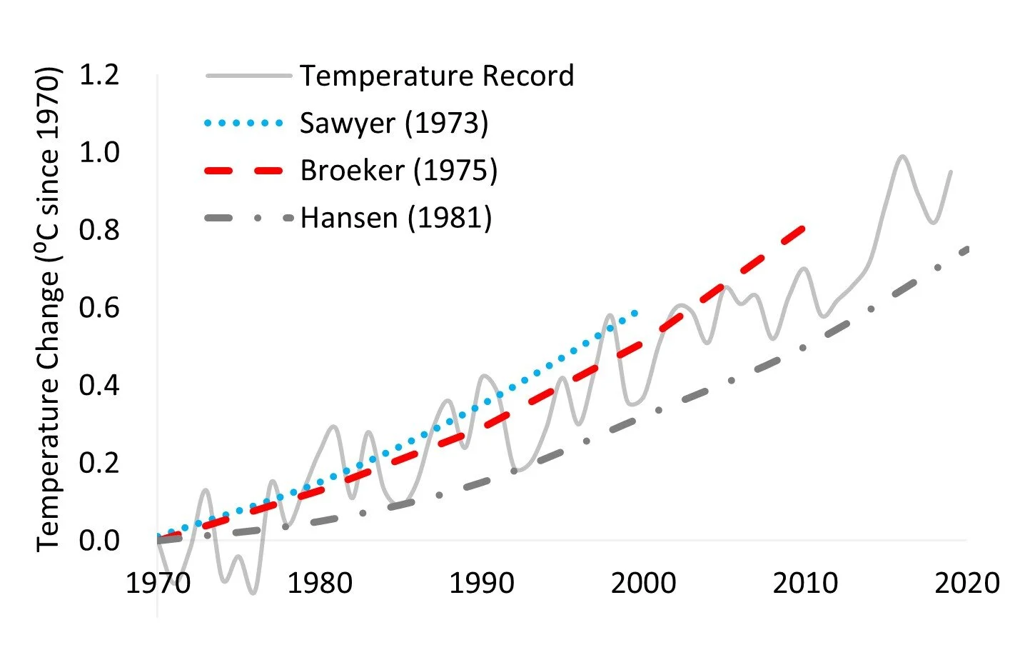
Have climate models correctly predicted global warming? Yes, even the earliest models (first run half a century ago) have proven highly accurate.
The Pioneering Swedish Chemist
In the late nineteenth century, scientists were piecing together a growing understanding of the intertwining role of CO2, the carbon cycle, and the sun’s energy and how these factors interacted with Earth systems to control the temperature and climate. Swedish chemist, Svante Arrhenius was the first to publish a mathematical basis for the greenhouse effect in his 1896 paper: “On the influence of carbonic acid {CO2} in the air upon the temperature of the ground”.
Arrhenius approached the problem in three stages. First, he calculated the amount of energy absorbed by carbon dioxide and water vapour using the best experimental evidence of the time. Next, he split the Earth into 13 sections by latitude and estimated the average reflection of sunlight from cloud, snow, ocean, and land in each slice for every month of the year. Finally, he assigned an initial amount of atmospheric water vapour to each cross section and built a formula to allow the absorption from water vapour to change with temperature.
Now all he needed to do was insert the energy inflow from the sun and the different concentrations of CO2 and he could calculate the planetary energy budget and temperature change.
Armed with only paper and pencil it took Arrhenius one year to crunch the numbers over six different CO2 scenarios; an arduous task which he only undertook as a distraction from his ongoing divorce from his former pupil, Sofia Rudbeck.
Once the year of distraction was up, he estimated that if the concentration of CO2 doubled, the Earth would warm by 5-6⁰C.
Whilst Arrhenius’ maths was sound, he was let down by the inaccuracy of the experimental absorption data and he missed some key physical changes such as the cooling impact of water evaporation from a warmer surface. This over-inflated his temperature estimates.
The Early Warnings of a British Engineer
Forty years later, British steam engineer Guy Stewart Callendar would rebuild Arrhenius’ mathematical model with the benefit of more accurate CO2 absorption recordings and a growing database of temperature and CO2 measurements.
He started by estimating that burning of fossil fuels were responsible for a 6% increase to CO2 between 1880 and 1930 and that temperatures had risen by 0.3⁰C through the same period. Next he built a similar mathematical representation of the climate to Arrhenius with fixed land, sea, ice, and clouds. He asserted that the increase in CO2 was responsible for half of the 0.3⁰C warming through the period.
This was the first time CO2 emissions from human activity had been linked to a recorded temperature increase of Earth. His model predicted that doubling CO2 in the atmosphere would increase temperatures by 1.6⁰C.
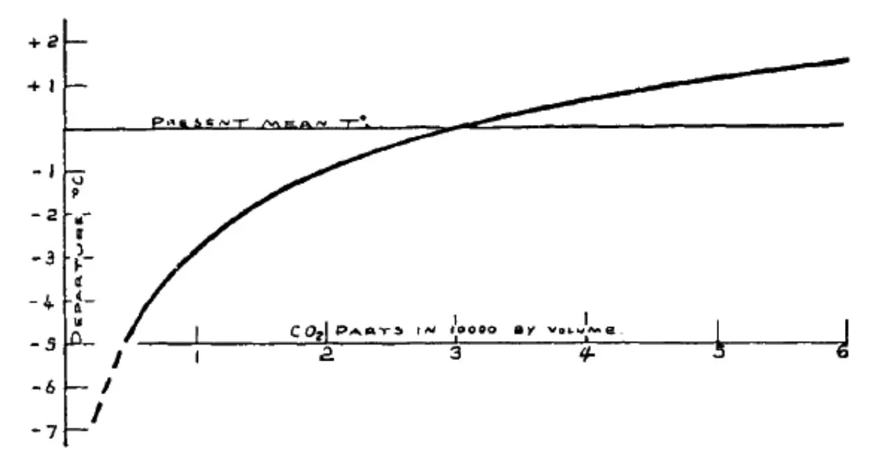
Original image from Guy Stewart Callendar’s 1938 paper “The Artificial Production of Carbon Dioxide and its Influence on Temperature”. Horizontal axis shows CO2 in parts per 10,000 (multiply by 100 for ppm). Vertical axis shows his predicted temperature change in ⁰C. The increasingly shallow curve shows a logarithmic relationship.
Where Arrhenius was let down by the accuracy of experimental data, Callendar decided not to model water vapour change with temperature increase. He captured the thermostat but missed the boost button and underestimated the overall temperature increase.
Simple But Effective
Both Arrhenius’ and Callendar’s models suffered from large oversimplifications, missing key feedbacks such as the amplifying effect of water vapour, the cooling impact of evaporation and changes to ice, clouds, and circulation. Nonetheless, by luck or intuition, the two estimates are broadly consistent with the upper and lower range of the best predictions today: a “very likely” temperature increase of between 2 and 5⁰C for double the atmospheric CO2 or a “likely” 2.5-4⁰C (IPCC AR6).
Arrhenius and Callendar had not only laid the foundations for modelling how energy gets trapped in the Earth system (radiative forcing) but also the relationship between CO2 concentrations and temperature. A relationship which is non-linear. They follow what mathematicians call a logarithmic relationship – the increasingly shallow curve of Callendar’s graph. The logarithmic relationship means that higher CO2 concentrations will always drive higher temperatures, but the increase in temperature for every extra unit of CO2 becomes smaller with increasing concentrations.
Doubling CO2 from 300 ppm to 600 ppm will give you roughly the same absolute temperature change as doubling CO2 from 600 to 1,200ppm. Why? Well, infrared absorption in the atmospheric window increases most as CO2 concentrations first rise – these are the easy pickings where CO2 can absorb in frequencies of the spectrum not already blocked by water vapour. But as concentrations of CO2 further increase, the infrared absorption also becomes increasingly saturated and only small further broadenings of the absorption band can trap extra energy.
Think of global warming like putting on weight; the more you eat the fatter you get, but as you get heavier it takes more and more calories to maintain your larger body so the weight gains eventually slow.
Upgrading to Smart Heating: Developing Climate Models
In 1967, Manabe and Wetherald published what is regarded as the cornerstone of contemporary climate modelling. They created the first computer simulation to represent the major radiative forcings (energy flows) and key feedback elements of Earth’s climate such as water vapour, evaporation, and clouds, in a one dimensional slice of the atmosphere.
They estimated doubling CO2 would bring 2.4⁰C temperature increases – this was the first scientifically convincing basis for the greenhouse effect. Since Manabe and Wetherald published that seminal paper, computing has grown exponentially and models have moved from one dimensional representations into a grid of three-dimensional cubes of atmosphere, land, sea ice, and ocean which interact with one another.
These complex models are called General Circulation Models (GCM) and can be used to predict the weather or the future climate.
Our weather is controlled by the flow of energy through the Earth system. The bulk of the sun’s energy enters Earth at the tropics and flows towards the poles, carried by wind, water currents, and influenced by the spin of the planet, finally escaping the atmosphere as infrared radiation. To predict the weather, simulations start at an exact state and must move to another exact state over an exact period of time. This limits meaningful weather forecasts to only ten days out.
However, climate is the probability of weather.
Climate models simulate land, oceans, atmosphere, and ice, using scientific principles established 100 to 300 years ago and used in all aspect of modern life.
Maxwell’s equations of light describe how the sun’s radiation enters the Earth and how infrared radiation leaves the atmosphere.
Thermodynamics models how energy interacts with the physical world, the same equations used to calculate the power output of a combustion engine.
Navier-stokes equations model the dynamic movement of air and water flowing across the planet just as they are used to predict how an aeroplane will fly.
These equations are combined in the grids of General Circulation Models and used to simulate the statistical average temperatures, velocities, and pressures of the Earth system far into the future. Modern climate models have one million lines of code which is relatively compact compared to Google Chrome which contains just over six million. The difference is that Google answers just one question at a time using one computer processor whereas climate models must cycle through 65,000 cubes of code every minute for hundreds of years. This requires super-computers with millions of processers using upto 5,000 kW power – the same as a small town.

Unsplash by Taylor Vick
Climate models are continually being refined and more feedback elements incorporated. Aerosols were added in the IPCC’s second assessment, the carbon cycle and dynamic vegetation by the third assessment and land ice, the ocean pump, and atmospheric chemistry through the third and forth assessments. The next generation of models are called Earth Systems Models (ESM) which will add further elements such as melting tundra, wildfires, wetlands, and land ice sheets.
Predicting Change
Whilst modelling and predicting climate is a highly complex feat, the underlying science is robust. We know the relationship between CO2 and temperature extends deep into geological time. Climate scientists can explain this relationship based on the fundamental physics, chemistry, and biology of the Earth system. And this scientific basis can be used to predict future temperature changes with even the earliest of these models (from the 1970s) proving highly accurate so far.
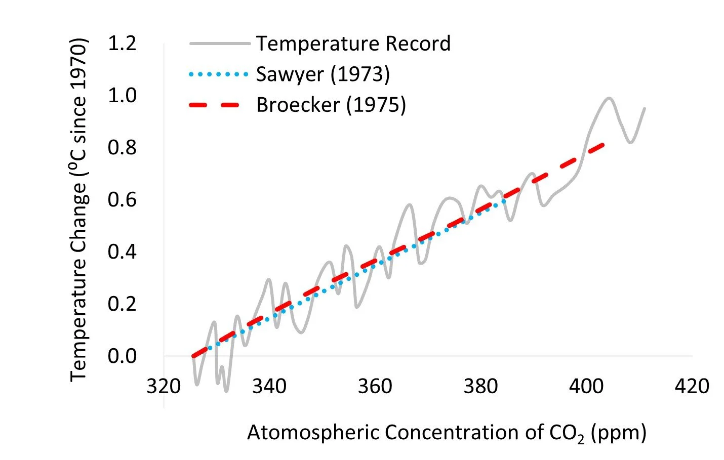
The same temperature predictions by Sawyer and Broecker but in relation to CO2 ppm concentrations rather than by year.